The Evolution of the Attention Mechanism in LLMs

Serving one 4,096-token request on Qwen3-32B takes about 1.07 GB of key-value cache. Give every query head its own keys and values, as the original Transformer did, and that same request would need 8.59 GB.

As a language model’s context grows, reading and storing its history becomes more expensive. Attention designs tackle different parts of that cost: some share keys and values across heads, some compress what each token stores, and others restrict which positions a query reads.

We’ll follow these choices from a single attention head to hybrid memory and paged caches, using small worked examples. The question throughout is simple: what changes, what does it save, and what do we give up?

1. Attention Was All We Needed?

A language model needs more than a representation of each token in isolation. It needs a way to bring information from the surrounding context into that representation. Attention provides that connection: each position computes weights over the context it can see, then uses those weights to combine information from those positions.

In a Transformer, this happens inside a block that also contains a feed-forward network. Stack these blocks, and the representations produced by one become the inputs to the next. In the decoder-only pattern used by GPT-style models, a vocabulary projection at the end produces scores for the next token.

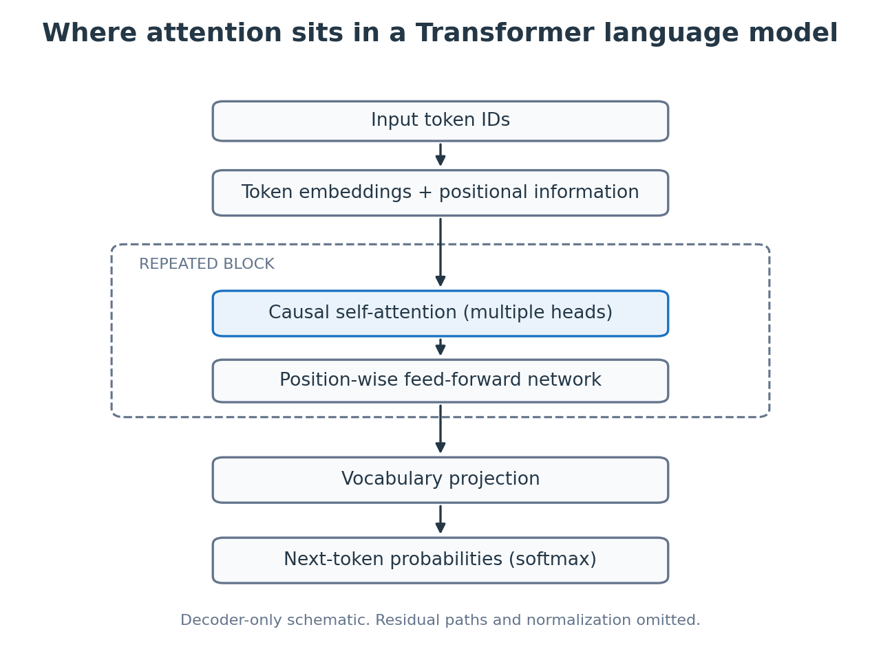Simplified decoder-only architecture; residual connections and normalization are omitted. Original schematic following Jay Alammar’s The Illustrated GPT-2.

An attention head is one learned query/key/value projection pathway within the attention layer. It produces its own weights for mixing token information. Multiple heads give the layer several such pathways in parallel. For a fuller introduction, Jay Alammar’s The Illustrated Transformer and The Illustrated GPT-2 cover the surrounding architecture in detail.

We’ll start with multiple heads, then explore shared KV caches, restricted reads and compressed representations. From there, we’ll look at output gates, hybrid memory and cache allocation. Each design addresses a different constraint, and a model can combine several of them.

The companion examples use small inputs to make the calculations and storage costs inspectable. They demonstrate how the mechanisms work. The weights are chosen by hand, not trained, so they say nothing about model quality, and none of the examples is a latency or throughput benchmark.

2. Single-Head Self-Attention

Start with one head. The original Transformer already used multiple heads, but isolating one lets us see the computation that the later designs modify.

Self-attention projects the input into queries, keys and values. Queries and keys determine how strongly positions match; values carry the information that gets mixed. The scaled dot-product formulation combines these operations:

\[\begin{aligned} Q &= XW_Q, \quad K = XW_K, \quad V = XW_V \\ A &= \operatorname{softmax}\!\left(\frac{QK^{\mathsf T}}{\sqrt{d_k}} + M\right) \\ Y &= (AV)W_O \end{aligned}\]

Here \(d_k\) is the query/key dimension. Scaling moderates dot-product growth with dimension, and softmax normalizes the scores across keys. For causal attention, \(M\) masks future positions before normalization, so each query reads only its own position and earlier ones.

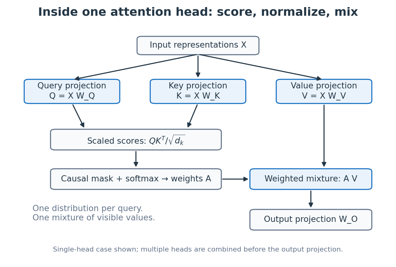One head computes a distribution over visible positions, mixes their values, and applies an output projection. Original schematic; see Alammar’s Q/K/V walkthrough and the Transformer paper.

For a concrete example, take “The cat sat” with chosen vectors \([1, 0]\), \([0, 1]\) and \([1, 1]\). Use identity projections so we can follow the calculation directly. These are untrained teaching vectors, with positional encoding omitted. The query for “sat” has dot products \([1, 1, 2]\) with the keys. Scaling and softmax turn these into weights of approximately \([0.248, 0.248, 0.503]\). Mixing the values gives \([0.752, 0.752]\).

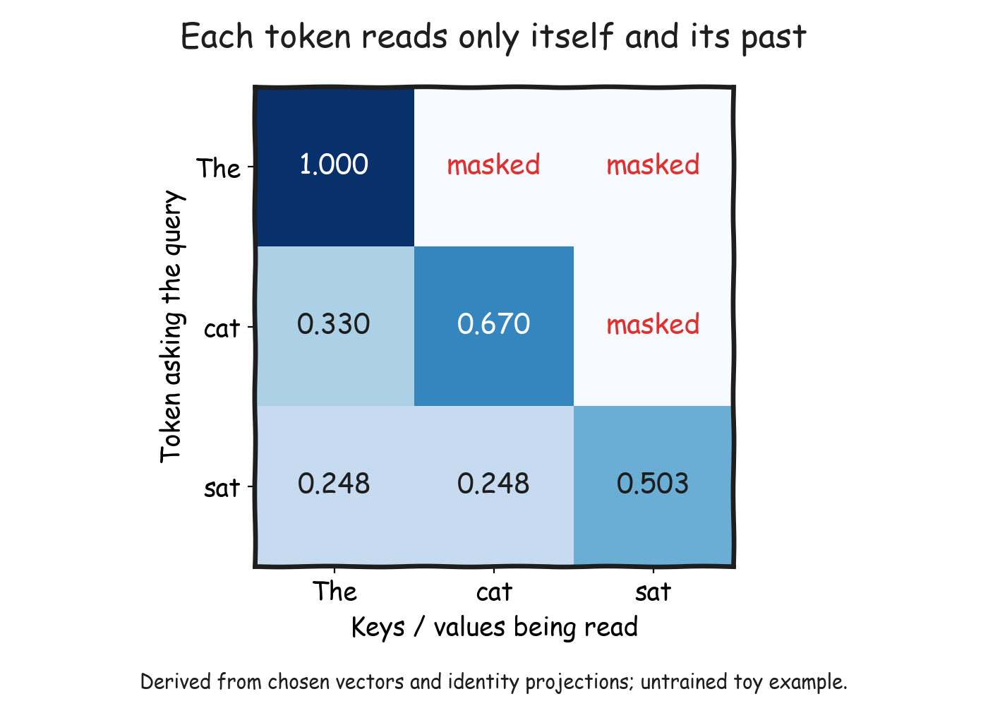Computed weights for the example: each row is a query, each column a key/value position. Future positions receive zero weight.

The result is a context-dependent mixture. To understand its cost, distinguish processing a sequence from generating one new token. Holding the head dimensions, batch size and numerical precision fixed:

Quantity	Growth with sequence length \(n\)	Why
Full-sequence attention work, as during prompt prefill	\(\mathcal{O}(n^2)\)	Each query attends to its visible keys
Attention work for one new token with a KV cache	\(\mathcal{O}(n)\)	The new query reads the retained history
Retained KV-cache storage	\(\mathcal{O}(n)\)	Each retained token contributes one key and value per head

Full-sequence attention has quadratically many query-key interactions, but implementations can avoid storing the entire score matrix at once. A KV cache reuses earlier keys and values during generation; the new query still has to read them. The runnable implementation and example show both full-sequence and cached execution.

There is another constraint: one head gives each query one attention distribution. Several relationships can contribute, but they share those mixing weights. Multiple heads let the layer form separate distributions through different learned projections, then combine their outputs. That is the first architectural change we’ll make.

Key Takeaways

• One head forms a context-dependent mixture of visible token representations.
• A causal mask excludes future positions; a KV cache reuses earlier keys and values during generation.
• Full-sequence attention work grows quadratically; one cached decoding step and retained KV storage grow linearly with history length.

3. Multi-Head Self-Attention

Single-head attention has a fundamental limitation: each query gets only one attention distribution. But language is rich with different types of dependencies—syntactic, semantic, positional, and more. Multi-head attention solves this by running multiple attention operations in parallel.

The Intuition

Think of the heads as specialists that can look for different patterns in the same context. Their roles are learned: one head can capture several relationships, and different heads can learn overlapping patterns.

Mathematical Formulation

The attention calculation stays the same. We now give each head its own learned query, key and value projections, then concatenate their outputs and apply a learned output projection:

\[\begin{aligned} \operatorname{head}_i &= \operatorname{Attention}(XW_Q^i, XW_K^i, XW_V^i) \\ \operatorname{MultiHead}(X) &= \operatorname{Concat}(\operatorname{head}_1, \ldots, \operatorname{head}_h)W_O \end{aligned}\]

The Transformer paper describes this as attending across different representation subspaces.

Let’s reuse “The cat sat” and the same input vectors. This time, split the two input coordinates across two heads: the first head projects onto the first coordinate, and the second onto the second. Each head therefore has width one, keeping the total width unchanged. These are chosen projections to make the difference visible, with positional encoding still omitted.

For the final query, the first head assigns weights of approximately \([0.422, 0.155, 0.422]\) to “The,” “cat” and “sat.” The second assigns \([0.155, 0.422, 0.422]\). Same input, different mixtures. Their scalar outputs are concatenated into \([0.845, 0.845]\); an identity output projection leaves that vector unchanged in this example.

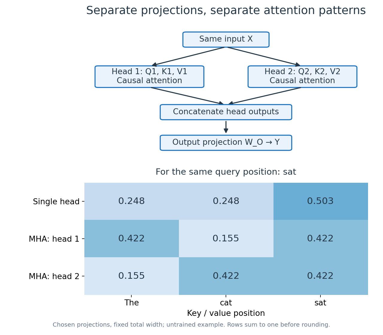The architecture above the heatmap shows how the head outputs are combined. The calculated weights below show the final query from our single-head example alongside the two narrower heads.

Putting the Heads to Work

We don’t need a Python loop for each head. The implementation packs their projections into larger linear layers, reshapes the result to expose a head dimension, and computes attention across those heads in a batch. The runnable example exposes the weights so we can inspect the patterns above.

What Does This Cost Us?

Here’s a detail that’s easy to miss: more heads do not automatically mean a larger KV cache. Usually, we divide a fixed model width across the heads. If \(h \times d_{\text{head}} = d_{\text{model}}\), changing the head count while keeping \(d_{\text{model}}\) fixed leaves the total cached width unchanged.

For equal key and value widths, the cache payload in bytes across the model is:

\[\begin{aligned} &2 \times \text{batch\_size} \times \text{cached\_length} \times \text{n\_layers} \\ &\quad \times h \times d_{\text{head}} \times \text{bytes\_per\_element} \end{aligned}\]

The cache still grows with context length, batch size and layer count. Each head retains its own keys and values, and each new query reads that history. Splitting into heads also keeps full-context attention quadratic in sequence length.

That leaves us with a useful question: do all those query heads need separate keys and values? Could they ask different questions while reading from shared memory? That is the idea behind multi-query attention.

Key Takeaways

• Separate projections let heads form different attention patterns, which are combined through an output projection.
• Packed projections and batched attention compute the heads together.
• At fixed total width, more heads do not automatically increase KV-cache size. Retaining separate keys and values for every head still leaves a memory cost worth reducing.

4. Sharing the KV Cache: MQA and GQA

Multi-head attention gives every head its own keys and values to store during generation. But do all those heads need separate memories? Multi-query attention (MQA) lets each head ask its own question through a separate query projection, while sharing one set of keys and values across all heads. With eight heads sharing one K/V set, for example, the KV cache becomes eight times smaller at the same head width. Reading less data at each decoding step can also mean lower latency.

MQA: One Shared KV Head

The query projections stay separate, but every head now reads the same keys and values. The causal mask and the way we combine outputs stay unchanged:

\[\begin{aligned} Q_i &= XW_Q^i, \quad K_s = XW_K, \quad V_s = XW_V \\ \operatorname{head}_i &= \operatorname{softmax}\!\left(\frac{Q_iK_s^{\mathsf T}}{\sqrt{d_k}} + M\right)V_s \\ \operatorname{MQA}(X) &= \operatorname{Concat}(\operatorname{head}_1, \ldots, \operatorname{head}_h)W_O \end{aligned}\]

This is the sharing strategy introduced in Noam Shazeer’s MQA paper. Shared memory still allows different attention distributions: in our “The cat sat” example, the query heads at “cat” assign \([0.500, 0.500]\) and \([0.731, 0.269]\) to the same visible positions. They read the same keys and values but ask different questions.

The catch is that all heads must work with one shared K/V representation. That restriction can affect quality, even though the queries remain separate. So what if we relaxed the sharing a little?

GQA: Share Within Groups

Instead of making every query head share one memory, give each group its own keys and values. With four query heads and two KV groups, heads 1 and 2 share one K/V pair, while heads 3 and 4 share another.

This is grouped-query attention, introduced by Joshua Ainslie and colleagues. For evenly sized groups, a query head selects its KV group as follows, using zero-based indices:

\[\begin{aligned} \text{group\_size} &= \left\lfloor \frac{\text{n\_heads}}{\text{n\_kv\_heads}} \right\rfloor \\ \text{group} &= \left\lfloor \frac{\text{head\_index}}{\text{group\_size}} \right\rfloor \\ \operatorname{head}_i &= \operatorname{Attention}(Q_i, K_{\text{group}}, V_{\text{group}}) \end{aligned}\]

Now we can describe all three designs with the same parameter:

Design	KV heads for \(h\) query heads	Sharing
MHA	\(h\)	Each query head has its own K/V
GQA	Between \(1\) and \(h\)	Query heads share within groups
MQA	\(1\)	All query heads share K/V

MQA is the one-group endpoint of GQA. They are choices along the same spectrum; applying both does not produce another round of cache savings.

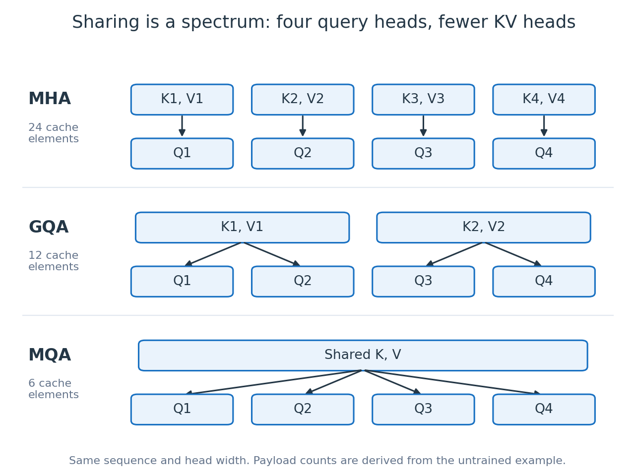Illustrative topology showing who shares with whom. Cache counts come from the same fixed-width, four-head example; the queries and sequence stay unchanged across designs.

To make an intermediate group count visible, our grouped example repeats the earlier input coordinates into a wider representation and uses four scalar query heads. Its K/V payload falls from 24 elements with MHA, to 12 with GQA, to 6 with MQA.

What Do We Save, and What Do We Give Up?

We can use one cache formula for the whole spectrum, assuming equal key and value widths:

\[\begin{aligned} \text{KV payload bytes} &= 2 \times \text{batch\_size} \times \text{cached\_length} \\ &\quad \times \text{n\_layers} \times \text{n\_kv\_heads} \\ &\quad \times d_{\text{head}} \times \text{bytes\_per\_element} \end{aligned}\]

Holding the other dimensions fixed, the reduction relative to MHA is \(\frac{\text{n\_heads}}{\text{n\_kv\_heads}}\). As a larger example, Qwen3-32B’s configuration has 64 query heads and 8 KV heads. At batch size 1 and 4096 cached tokens, its 64 layers and head width 128 give a derived BF16 cache payload of 1.07 GB, versus 8.59 GB for a hypothetical MHA version: an 8× reduction. These are decimal gigabytes of K/V data, excluding weights, temporary tensors and allocator overhead.

The quality and latency tradeoff is less mechanical. The GQA study found quality close to MHA with inference speed close to MQA in its evaluated settings. Converting existing checkpoints also involved further training. Group count gives us a design choice, not a universal optimum or a free inference-time swap.

Our implementations retain only the KV groups in the cache. The GQA path uses an explicit group dimension so adjacent query heads read the right group without an explicit per-query KV repetition. Backend temporaries and kernel selection still matter.

Where These Show Up

Design	Model examples	Primary source
MHA	GPT-2	OpenAI’s implementation
MQA	PaLM; Falcon-7B	PaLM paper; Falcon-7B configuration
GQA	Llama-2-70B; Llama-3-8B and 70B	Meta’s model configurations
GQA	Falcon-40B; Mistral-7B v0.1	Falcon-40B configuration; Mistral paper
GQA	Qwen3-32B	Qwen3-32B configuration

These labels apply to the named variants, not necessarily their entire model families. Mistral-7B also combines GQA with sliding-window attention, which changes a different part of the problem: how many token positions each query reads.

Key Takeaways

• MQA and GQA keep separate queries while sharing keys and values across all heads or within groups.
• MHA, GQA and MQA form a spectrum controlled by the number of KV heads; their cache reductions do not stack.
• Fewer KV heads reduce stored history, with quality and latency tradeoffs that depend on training and execution.
• Sharing heads still leaves the sequence-length cost. Sliding-window attention tackles that next.

5. Sliding Window Attention

GQA reduces the number of KV heads, but each query still reads the retained sequence. As the context grows, so does the work. Sliding-window attention, used for long documents in Longformer, changes a different part of the problem: how far back each query looks.

The Intuition

Do tokens really need to attend to every previous token? Often, much of the useful context is nearby. Give each query a window of recent positions instead of the entire history. Here, the window size \(W\) includes the current position, so a query at position \(i\) can read:

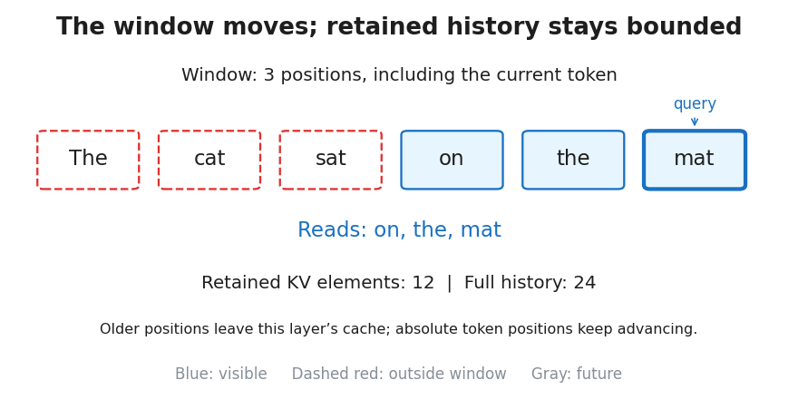
\[\max(0, i - W + 1) \leq \text{key\_position} \leq i\]

Let’s extend our sentence to “The cat sat on the mat” and use a window of three positions. The query at “sat” can read “The cat sat.” Move to “on,” and the window becomes “cat sat on.” At “mat,” it reads only “on the mat.” The attention calculation within that window is unchanged; older positions simply stop participating.

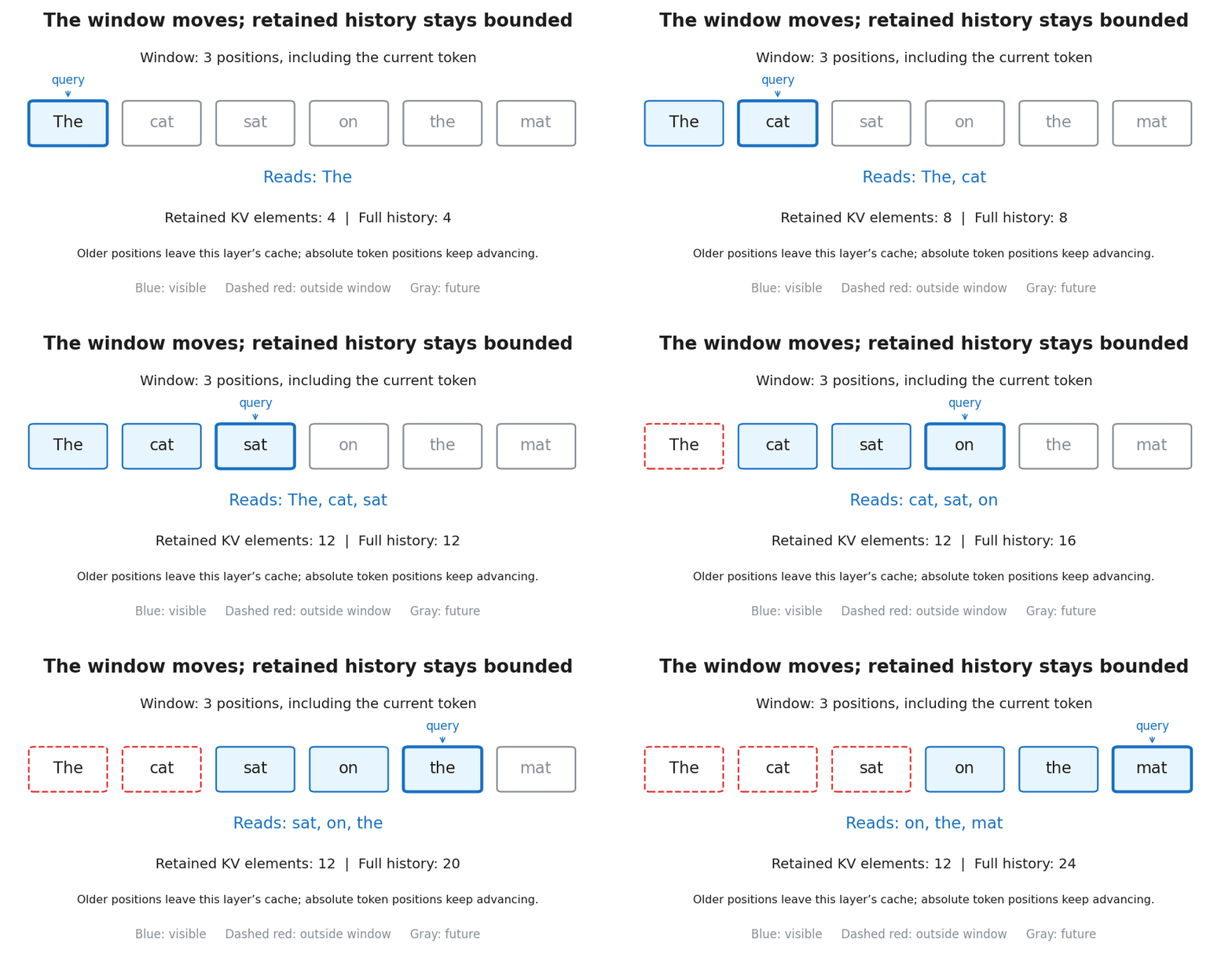Visibility and cache counts follow the verified single-layer example. Static version.

What Changes in the Cost?

Full causal attention has quadratically many query-key pairs across a sequence. With local execution, each query reads at most \(W\) positions, reducing that attention work to \(\mathcal{O}(nW)\) for sequence length \(n\). For a fixed window, that is linear in sequence length. In our six-token example, the number of visible pairs per head falls from 21 to 15; the gap grows with longer sequences.

That benefit requires computing only the local interactions. Creating a dense score matrix and masking most of it afterward still does the dense computation. Our implementation processes local slices directly. The example runner compares full-sequence and cached local execution.

Combining It with GQA

These two changes do compose: GQA reduces the number of KV heads, while a rolling window bounds the retained positions per local layer. Once the window fills, older K/V entries can leave that layer’s cache. Its retained payload is:

\[\begin{aligned} &2 \times \text{batch\_size} \times \min(\text{cached\_length}, W) \\ &\quad \times \text{n\_kv\_heads} \times d_{\text{head}} \times \text{bytes\_per\_element} \end{aligned}\]

The token position keeps advancing even when the stored length stops growing. A rolling cache reuses its slots, but positional encoding still uses each token’s true position, so a cache slot and a token’s position are no longer the same number.

What Do We Give Up?

An older token can no longer be read directly by that local layer once it leaves the window. That can matter when a task needs information from far back. Stacked layers can relay information over longer distances, however, so the per-layer window is not the model’s entire effective context.

Mistral-7B v0.1 combines GQA with sliding-window attention; its configuration specifies a window of 4096. Gemma 2 takes another approach, alternating local sliding-window and global attention layers. Those global layers still need their broader history, so the bounded-cache formula above applies to the local layers.

Key Takeaways

• Sliding-window attention restricts token positions; GQA shares KV heads. Their savings address different dimensions.
• Local execution makes attention work \(\mathcal{O}(nW)\) and a rolling cache bounds retained history per local layer.
• The tradeoff is reduced direct access to distant tokens; stacked layers and local/global designs can provide broader information paths.

A window is a simple rule for deciding what to read. But what if the useful token is somewhere much earlier?

6. Sparse Attention Beyond Sliding Windows

A sliding window assumes recent tokens deserve our attention. Often they do. But if a function was defined two thousand tokens ago, a wider window is a fairly expensive way to find it again. Can we keep the local context and selectively reach further back?

Sparse attention is a family of answers: local bands, designated global positions, selected blocks, or tokens chosen from their content. The common idea is to spend the full attention calculation on a subset of the history. The selection rule determines what the layer can miss.

For a local window plus selected remote tokens, the calculation becomes:

\[\begin{aligned} S_t &= \operatorname{local\_window}(t) \cup \operatorname{selected\_remote\_tokens}(t) \\ \operatorname{output}_t &= \operatorname{softmax}\!\left(\frac{q_t K[S_t]^{\mathsf T}}{\sqrt{d}}\right)V[S_t] \end{aligned}\]

Both sets contain only positions up to the current token, so their union \(S_t\) already enforces causal visibility.

Our example gives each query two local positions, including itself, and one remote slot. When reading “mat” in “The cat sat on the mat”, the chosen index projections select the first “The” as well as the final “the mat”: positions [0, 4, 5]. That distant token is directly visible again.

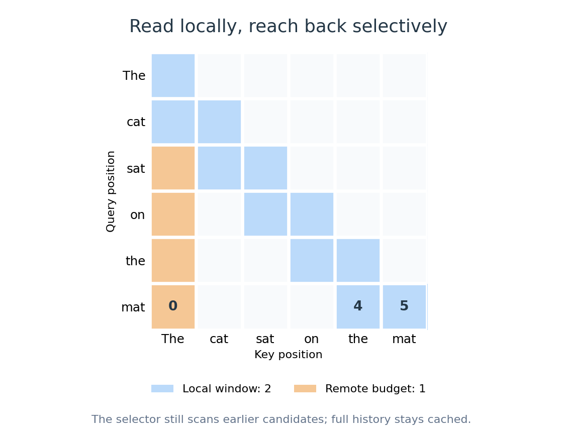Blue cells are local reads; orange cells are selected remote reads. White cells are skipped by the main attention calculation.

With window \(W\) and remote budget \(k\), the main attention stage reads at most \(W + k\) positions per query. Finding them has a cost too: our small indexer scans the earlier history, so selection can still take quadratic total work during prefill. It also retains the full K/V and index-key history. Fewer attention reads do not automatically mean a bounded cache or an end-to-end speedup.

Native Sparse Attention combines compressed, selected and local branches. DeepSeek-V3.2-Exp uses DeepSeek Sparse Attention (DSA), with an indexer selecting entries for sparse attention. Our local-plus-selector implementation isolates selection rather than reproducing these architectures.

Compress First, Then Select or Reuse

So far, we’ve selected individual tokens. We can also compress groups of tokens into fewer entries, then decide which of those entries to read:

Token history → compressed entries → selected compressed entries

Illustrative sequence-compression path. Compression reduces the number of historical entries; selection limits which entries a query reads.

DeepSeek-V4 combines a local window over uncompressed tokens with two forms of compressed history: Compressed Sparse Attention (CSA) selects from compressed entries, while Heavily Compressed Attention (HCA) reads all entries in a much more compressed history. The model interleaves these layer types. Compression now acts along the sequence dimension: fewer historical entries, with some detail traded for compact summaries.

DeepSeek-V4.1-Flash asks another question: does every layer need to repeat the same selection work? Its Compressed Sparse Attention 2 (CSA2) lets layers share cached representations and reuse selection results. Later decoder layers can also narrow their search to candidates found earlier, though finding that initial pool still has a cost.

For the curious: how CSA2 reuses work

CSA2 assigns layers Full, Reindex or Reuse modes, sharing KV and indexer keys and reusing top-k selections. A hierarchical indexer limits later decoder selection to an earlier candidate pool.

The progression is useful: choose fewer entries, compress those entries, then avoid rebuilding the same cache and selections at every layer. Our toy demonstrates the first step; these newer models combine several steps.

Key Takeaways

• Sparsity can preserve direct access to selected distant tokens while limiting the main attention reads.
• Selection cost, retained cache and hardware execution determine the actual savings; newer designs also compress history and reuse state across layers.
• Missing a useful token is the architectural tradeoff; choosing well requires more than a small attention budget.

MLA takes a different compression axis: shrink each token’s stored representation, rather than combine entries across time.

7. Multi-Head Latent Attention (MLA)

We’ve shared the KV heads and limited how much history each layer reads. Multi-head latent attention, introduced in DeepSeek-V2, changes what we store for each token: a compact learned representation from which the heads’ keys and values can be recovered.

The Key Idea

Instead of caching expanded K and V vectors, project each input into a smaller latent vector \(C\). Each head then has its own up-projections from that latent into content keys and values:

\[\begin{aligned} C &= XW_{\text{down}} \\ K_i &= CU_K^i, \quad V_i = CU_V^i \end{aligned}\]

The shared part is the latent state. The reconstructed keys and values can differ across heads, so this has a different constraint from making heads use identical K/V as in MQA. The model learns to work through this compact representation during training; it is not a lossless codec for an arbitrary existing MHA model.

Take “cat” from our four-head example. With the chosen down-projection, its latent is \([0, 1]\). The key up-projections produce \([0, 1, 1, -1]\), while the value up-projections produce \([1, 0, 1, 1]\), with one scalar per head. The three-token content cache stores 6 elements instead of 24 expanded K/V elements. Positional encoding is omitted in this worked example.

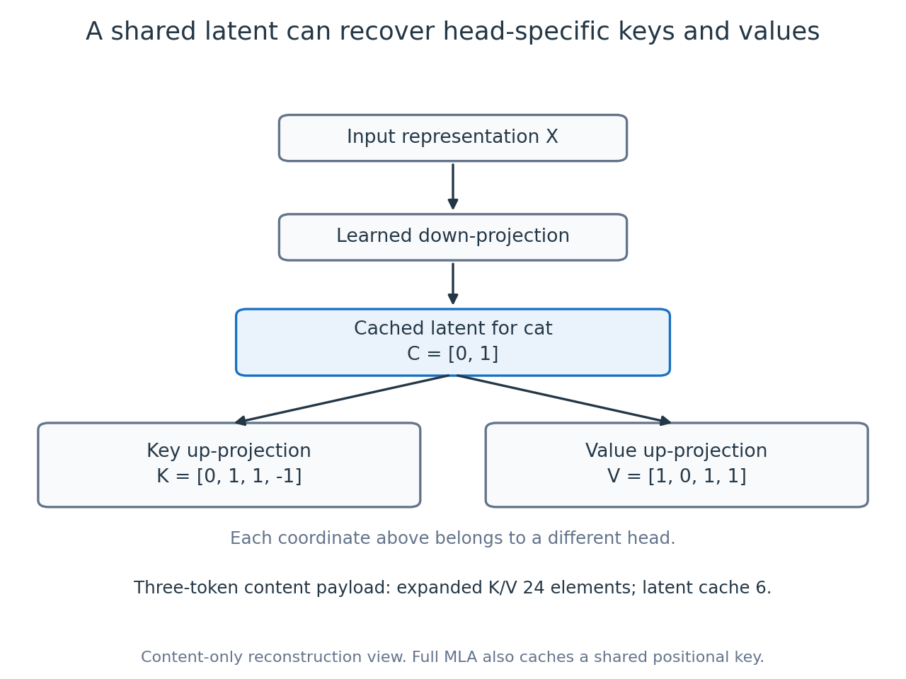Calculated reconstruction for the chosen vectors and weights. The diagram shows the content branch; positional information gets a separate path in the full design.

Do We Have to Decompress the Whole History?

That would give back some of the memory benefit as repeated work. Fortunately, we can rearrange the content calculation. For head \(i\), let \(Q_i\) be the current token’s content query and \(A_i\) its attention weights over the visible history. \(C\) holds the cached latent vectors, one row per token. Then:

\[\begin{aligned} Q_i(CU_K^i)^{\mathsf T} &= \bigl(Q_i(U_K^i)^{\mathsf T}\bigr)C^{\mathsf T} \\ A_i(CU_V^i) &= (A_iC)U_V^i \end{aligned}\]

These identities cover the content calculation; we’ll handle positional information next. For keys, move the up-projection into the current query before comparing it with the latent history. For values, mix the latents first and apply the up-projection afterward. The results match explicit reconstruction for the same factorized weights. This is the matrix-absorption idea: we can avoid rebuilding every past token’s expanded content keys and values during decoding.

Our implementation includes both paths, and the example compares them. The tradeoff depends on latent rank, head dimensions and kernels.

Where Does Position Information Go?

RoPE applies position-dependent rotations, which prevents us from freely moving a content up-projection through that rotation. DeepSeek’s solution is a decoupled positional branch: rotate a small query component and a shared positional key, then add their dot product to the content score.

That positional key is cached alongside the latent. For a layer with latent rank \(r\) and positional-key width \(d_{\text{rope}}\), the retained payload is:

\[\begin{aligned} &\text{batch\_size} \times \text{cached\_length} \\ &\quad \times (r + d_{\text{rope}}) \times \text{bytes\_per\_element} \end{aligned}\]

So the full cache is more than just \(C\), and it still grows with context length. Our educational model implements this decoupled RoPE path and causal cached decoding, while omitting the production model’s query bottleneck and normalization layers. Its cache allocates only the latent and positional buffers.

Where This Is Used

DeepSeek-V2 introduced MLA, and DeepSeek-V3 retained it. The compression ratio is an architectural choice: a smaller latent imposes a stronger constraint on what the heads can reconstruct. Training determines how well the model uses that capacity.

Key Takeaways

• MLA shares a compact latent while retaining head-specific content K/V up-projections.
• Matrix absorption avoids explicitly reconstructing the entire content K/V history during decoding.
• Full MLA also retains a shared positional key; cache savings depend on both latent rank and positional width.
• Compression reduces the stored representation, while context length, model quality and execution cost remain separate considerations.

8. Gated Softmax Attention

So far, we’ve changed what attention reads or stores. Here’s a different question: once a head has read the context, how much of its answer should it pass on?

Softmax distributes a total weight of one across the visible keys. Even when a head’s retrieved information is unhelpful, it still produces that weighted mixture. A learned gate gives the model another control: scale the retrieved output before mixing the heads together.

A simple head-wise version uses the same causal mask \(M\) as before:

\[\begin{aligned} H_i &= \operatorname{softmax}\!\left(\frac{Q_iK_i^{\mathsf T}}{\sqrt{d}} + M\right)V_i \\ g_i &= \operatorname{sigmoid}(Xw_{\text{gate}}^i + b_i) \\ Y &= \operatorname{concat}(g_1 \odot H_1, \ldots, g_h \odot H_h)W_O \end{aligned}\]

Each token gets one scalar gate per head, scaling every channel of that head’s output. Here \(\odot\) denotes elementwise multiplication, with the scalar applied across all channels. More expressive variants give individual output channels their own gates. The gate sits after the attention mixture and before the output projection; it does not replace softmax or renormalize the attention weights.

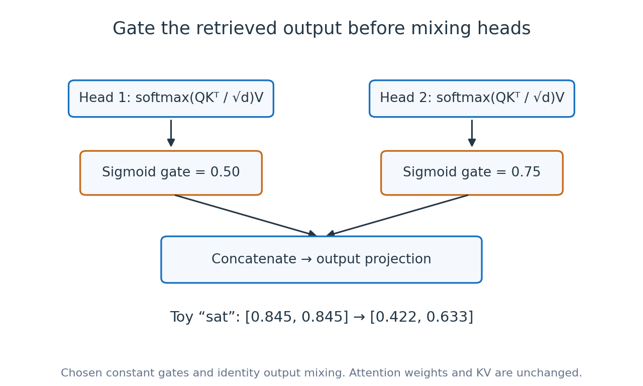The example fixes the gates to make their effect visible. In a trained model they depend on the current token representation.

For “sat” in our two-head example, the ungated output is \([0.845, 0.845]\). With identity output mixing and gates 0.50 and 0.75, it becomes [0.422, 0.633]. The attention distributions are unchanged; only the head outputs are scaled. The implementation also supports token-dependent gates and cached decoding.

Qiu and colleagues studied where to place these gates and reported training-stability and performance benefits for gating after scaled dot-product attention in their experiments. Qwen3-Next uses gated attention alongside Gated DeltaNet layers. Gating introduces input-dependent nonlinearity.

Key Takeaways

• Gated softmax controls how much of an attention output passes forward.
• Small output gates do not imply skipped token reads, less KV storage or a faster kernel.
• Output gating and sparse token selection solve different problems and can coexist.

9. Hybrid Attention: Mix Memory with Retrieval

Do all layers need to keep every token’s keys and values? A recurrent layer offers a different deal: update a fixed-size state as tokens arrive, then read from that state. The memory stays compact, but individual past tokens are no longer separately addressable.

Hybrid architectures combine these recurrent or linear-attention layers with softmax attention. Many layers can maintain compact state, while selected attention layers retain direct access to token history. We already saw a simpler kind of hybrid in Gemma 2’s local/global layout; here the mix changes the form of memory itself.

Gated DeltaNet updates its memory in two steps: first decay the existing state, then correct what it stores for the current key using the incoming value. Both steps update the same fixed-size matrix.

For the curious: the gated-delta update

For normalized keys and queries, our reference recurrence is:

\[\begin{aligned} S_{\text{decayed}} &= \alpha_t S_{t-1} \\ \operatorname{error}_t &= v_t - k_t^{\mathsf T}S_{\text{decayed}} \\ S_t &= S_{\text{decayed}} + \beta_t k_t \operatorname{error}_t^{\mathsf T} \\ \operatorname{output}_t &= q_t^{\mathsf T}S_t \end{aligned}\]

\(\alpha\) controls forgetting; \(\beta\) controls how strongly to correct the current association.

Repeated updates share the matrix’s capacity, so it is not an exact replacement for a list of past K/V vectors.

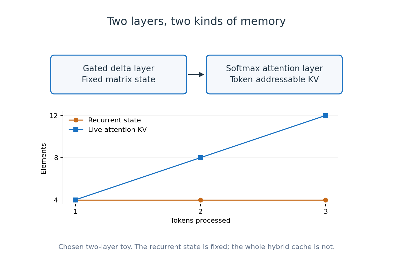Our two-layer example isolates the two kinds of memory. Counts are live tensor elements, not measured process memory.

The companion code puts one gated-delta layer before one ordinary attention layer. Across three tokens, its recurrent state stays at 4 elements, while the attention layer’s live KV grows 4 → 8 → 12. Full-sequence and cached execution agree. The whole hybrid therefore still has growing memory; only its recurrent component is fixed in context length.

Qwen3-Next-80B-A3B uses three Gated DeltaNet layers for every gated-attention layer, with MoE blocks in between. Our two-layer reference omits those blocks, convolutions, normalization and model-specific gate parameterization.

Kimi Linear makes another choice: combine Kimi Delta Attention (KDA) with MLA layers. KDA extends Gated DeltaNet with finer-grained gating, giving the recurrent state more selective control over forgetting. MLA supplies the layers that still read token history directly. This connects two ideas we’ve already covered: a hybrid can combine recurrent memory with compressed attention, rather than ordinary full attention. Our scalar-decay recurrence illustrates the shared foundation; it does not implement KDA’s finer-grained gates.

Key Takeaways

• Hybrid models choose which layers need token-addressable history and which can use compact recurrent state.
• Fixed state reduces history storage in recurrent layers, with a capacity and retrieval tradeoff.
• Remaining attention layers still grow their KV cache, even with MLA compression; both the layer mix and the attention design matter.

10. PagedAttention: Where the Cache Lives

Even after choosing a smaller cache, we still have to fit many requests into GPU memory. They arrive at different times, grow at different rates and sometimes share a prompt. Reserving a large contiguous cache for each request can waste capacity that another request could use.

PagedAttention, introduced with vLLM, brings paging to KV storage. Split each request’s logical token sequence into fixed-size blocks, then map those blocks to physical cache pages wherever space is available. The attention implementation follows a block table instead of requiring one contiguous history.

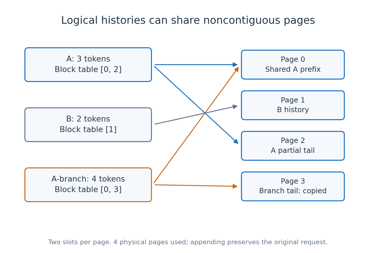Two tokens per page in our allocator example. Page numbers are storage addresses; their order does not change token positions.

Our reference allocator interleaves two requests, so A’s three tokens occupy pages [0, 2], while B occupies page 1. Forking A initially shares its pages. Appending to that branch copies the shared, partially filled final page before writing: the branch now uses [0, 3], and A’s history stays intact. This is copy-on-write; completed prefix pages can remain shared.

The softmax still covers the same visible keys. Our attention routine combines page-wise scores using a stable running maximum, denominator and weighted-value sum; its result matches a contiguous reference. Paging changes allocation and access, not which tokens the model attends to.

The payoff is at serving time: less reservation and fragmentation waste, plus reusable shared prefixes, can leave room for more concurrent requests. There is still page-table overhead and unused space in partially filled pages. Our CPU example verifies allocation, sharing and exact attention arithmetic. PagedAttention belongs to the serving stack rather than to a particular model architecture.

Key Takeaways

• PagedAttention maps logical KV history onto noncontiguous physical blocks.
• Prefix sharing and copy-on-write reduce duplication while preserving separate request histories.
• It preserves the attention calculation; savings come from managing cache capacity across requests.

11. A Brief Look Ahead

Efficiency is only part of the story. Differential Attention combines two softmax attention maps subtractively, giving it a way to cancel shared signals. Differential Transformer V2 revises this with a token-dependent, per-head subtraction gate and an implementation that uses standard FlashAttention kernels. Compare that with gated softmax: one scales a retrieved output; the other subtracts a learned fraction of another attention output. These are different ways to control what survives retrieval.

Attention Residuals (code) changes the axis of attention itself. Instead of only asking which earlier tokens matter, a layer learns how to mix earlier layers’ representations at the same token position. Its block variant groups layer outputs to reduce the overhead of retaining them all. This changes information flow through model depth and can sit alongside the token-attention mechanisms above.

12. Closing Thoughts

The interesting part of these designs is how many decisions fit inside the same query–key–value idea. We can share the history across heads, compress what represents it, choose which parts to read, or decide how much of the retrieved output to pass forward. We can also give different layers different kinds of memory, then organize that memory across requests at serving time.

Here’s the comparison of the attention designs we discussed:

Design	What changes	What it helps with	What to watch
Multi-head attention	Multiple learned query, key and value projections	Representing different relationships in parallel	Full-history attention still reads a growing token history
MQA / GQA	Query heads share KV heads	KV storage and repeated KV reads	Shared KV reduces independent per-head capacity
Sliding window	Each local layer reads recent positions	Bounded local history and attention work	Distant tokens lose direct visibility in that layer
Selected / compressed sparse attention	Select historical entries, optionally after sequence compression	Expensive attention over long histories	Selection overhead and information missed or compressed away
MLA	Cache a compact latent and positional key per token	Stored width of the history	Latent capacity, positional state and kernel design
Gated softmax	Scale retrieved outputs before mixing heads	Control over which retrieved features pass forward	Gating alone does not reduce token reads or KV storage
Recurrent / attention hybrids	Mix compact recurrent state with token-addressable attention	History storage in recurrent layers	Finite-state capacity and growing KV in the remaining attention layers
PagedAttention	Map logical KV history to physical pages	Allocation waste and duplicated prefixes across requests	Page management and partially filled blocks

These choices compose. GQA can sit inside a sliding-window layer; a hybrid can use MLA for its attention layers; a serving engine can page the resulting cache. The newer designs also make reuse across layers part of the architecture. Each choice changes a different part of the memory and computation budget.

The companion examples make those choices inspectable with the same small inputs.

When reading the next model report, start with three questions: what history is stored, which entries does a query read, and what work is repeated as the sequence grows? Then check how those choices map to the target hardware. Cache size and attention complexity explain part of generation throughput; kernels, batching and data movement determine how much of that advantage reaches the user.

References

• Attention Is All You Need (Vaswani et al., 2017)
• Fast Transformer Decoding: One Write-Head is All You Need (Shazeer, 2019)
• GQA: Training Generalized Multi-Query Transformer Models from Multi-Head Checkpoints (Ainslie et al., 2023)
• Qwen3 Technical Report (Qwen Team, 2025)
• Longformer: The Long-Document Transformer (Beltagy et al., 2020)
• Mistral 7B (Jiang et al., 2023)
• Gemma 2: Improving Open Language Models at a Practical Size (Gemma Team, 2024)
• DeepSeek-V2: A Strong, Economical, and Efficient Mixture-of-Experts Language Model (DeepSeek-AI, 2024)

• DeepSeek-V3 Technical Report (DeepSeek-AI, 2024)

• Native Sparse Attention (Yuan et al., 2025)
• DeepSeek-V3.2-Exp (DeepSeek-AI, 2025)
• Gated Attention for Large Language Models (Qiu et al., 2025)
• Gated Delta Networks: Improving Mamba2 with Delta Rule (Yang et al., 2025)
• Qwen3-Next-80B-A3B model card (Qwen, 2025)

• Efficient Memory Management for Large Language Model Serving with PagedAttention (Kwon et al., 2023)

• DeepSeek-V4: Towards Highly Efficient Million-Token Context Intelligence (DeepSeek-AI, 2026)
• DeepSeek-V4.1-Flash model card (DeepSeek-AI, 2026)
• Kimi Linear: An Expressive, Efficient Attention Architecture (Kimi Team, 2025)
• Differential Transformer (Ye et al., 2024)
• Differential Transformer V2 (Ye et al., 2026)
• Attention Residuals (Kimi Team et al., 2026)